Jahaan Bhavsar · student engineer

Jahaan’s Workspace

A maker driven by his endless questions about how things work.

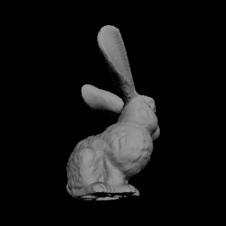
rasterix.js · 10,663 triangles

ORION · design, not yet built

01 Investigations

Software that shows its working.

Renderers and simulations,
built from the equations up.

Rasterix

How does a triangle become a pixel?

Java

Filled 968 triangles
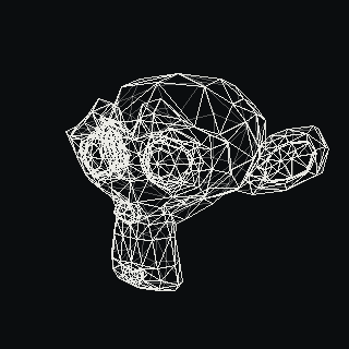
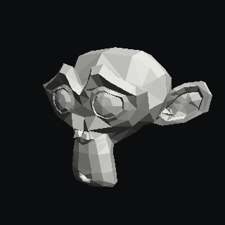
The mesh as points: its 507 vertices projected onto the screen. The projected triangles drawn as lines. Filled, depth-tested and flat shaded.
Drag to turn · point at a pixel
  1. x′ = (f/a)·x / w   y′ = f·y / w

    Divide by depth: far points move toward the centre. That is perspective.

    f = 1 / tan(fov/2)  ·  w = −zcam

  2. Eab(p) = (p − a) × (b − a)

    A pixel is inside when it sits on the same side of all three edges. The same three numbers become its weights.

    wᵢ = E / area  ·  inside when all wᵢ ≥ 0

  3. z = w0za + w1zb + w2zc

    Blend the corner depths with those weights, and draw only if nothing nearer is already there.

    kept only if nearer than the z-buffer

  4. k = 0.16 + 0.84·max(0, n̂·l̂)

    A face turned toward the light is brighter. The dot product measures how directly it faces it.

    n̂ from the cross product of two edges

u = w1u1 + w2u2 + w3u3
texel = (u(W−1), (1−v)(H−1))
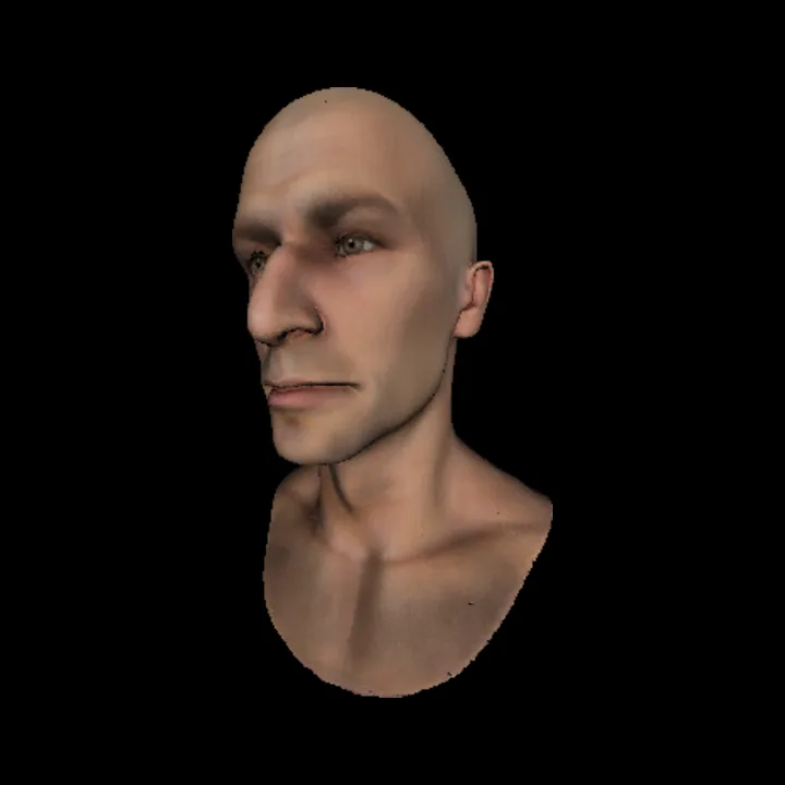
Each pixel reuses the weights it was drawn with to look up its colour in the image.
A textured human head rendered by Rasterix.
p0 = 2Δy − Δx
p ≥ 0 ? p += 2Δy − 2Δx : p += 2Δy
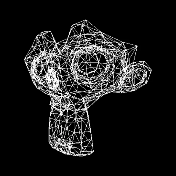
Bresenham: step one pixel in x; an integer error term decides when to step in y.
The same head as a wireframe in Rasterix.
n = (v2 − v1) × (v3 − v1)
s = 0.9 · n̂·l̂,  l̂ = (0, 0, −1)
One normal per triangle from a cross product; brightness is how squarely it faces the light.
The Stanford bunny, shaded, rendered by Rasterix.

Working prototype updated

QuantumSim

Probability you can walk around.

JavaScript · Three.js

P = |ψ(r)|² dV

Radial probability of the hydrogen 1s, 2s and 2p states Hand-drawn plot of P(r) = r squared times the radial wavefunction squared, against r in Bohr radii from 0 to 14. 1s peaks at r = 1, 2p at r = 4, and 2s has a node at r = 2 and its main peak near r = 5.2. 0 2 4 6 8 10 12 14 1s 2s 2p r / a₀ P(r) = r²|R(r)|²

the cloud is a sample, not a shell

Working prototype updated

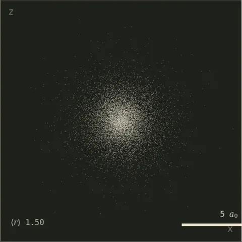
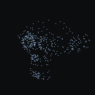
1s orbital: a round cloud of points, densest at the centre.
1s ⟨r⟩ = 1.5 a₀
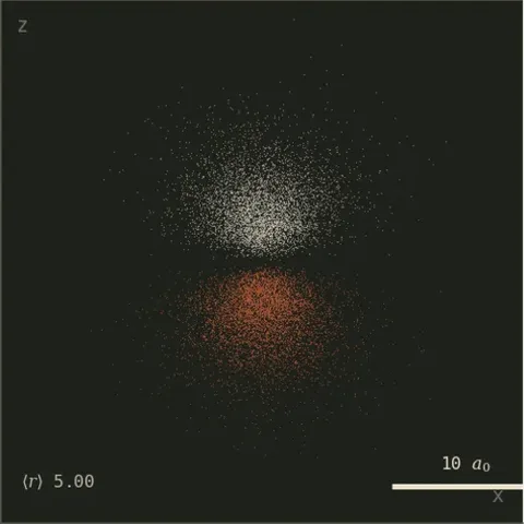
2p_z orbital: two lobes of opposite sign above and below one nodal plane.
2pz ⟨r⟩ = 5 a₀
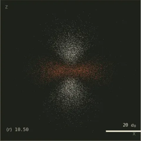
3d_z² orbital: two lobes along z with a ring of opposite sign around the middle.
3dz² ⟨r⟩ = 10.5 a₀
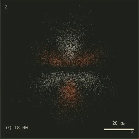
4f_z³ orbital: lobes and rings stacked along z, alternating in sign.
4fz³ ⟨r⟩ = 18 a₀

⟨r⟩ = (a₀/2)·(3n² − l(l+1))

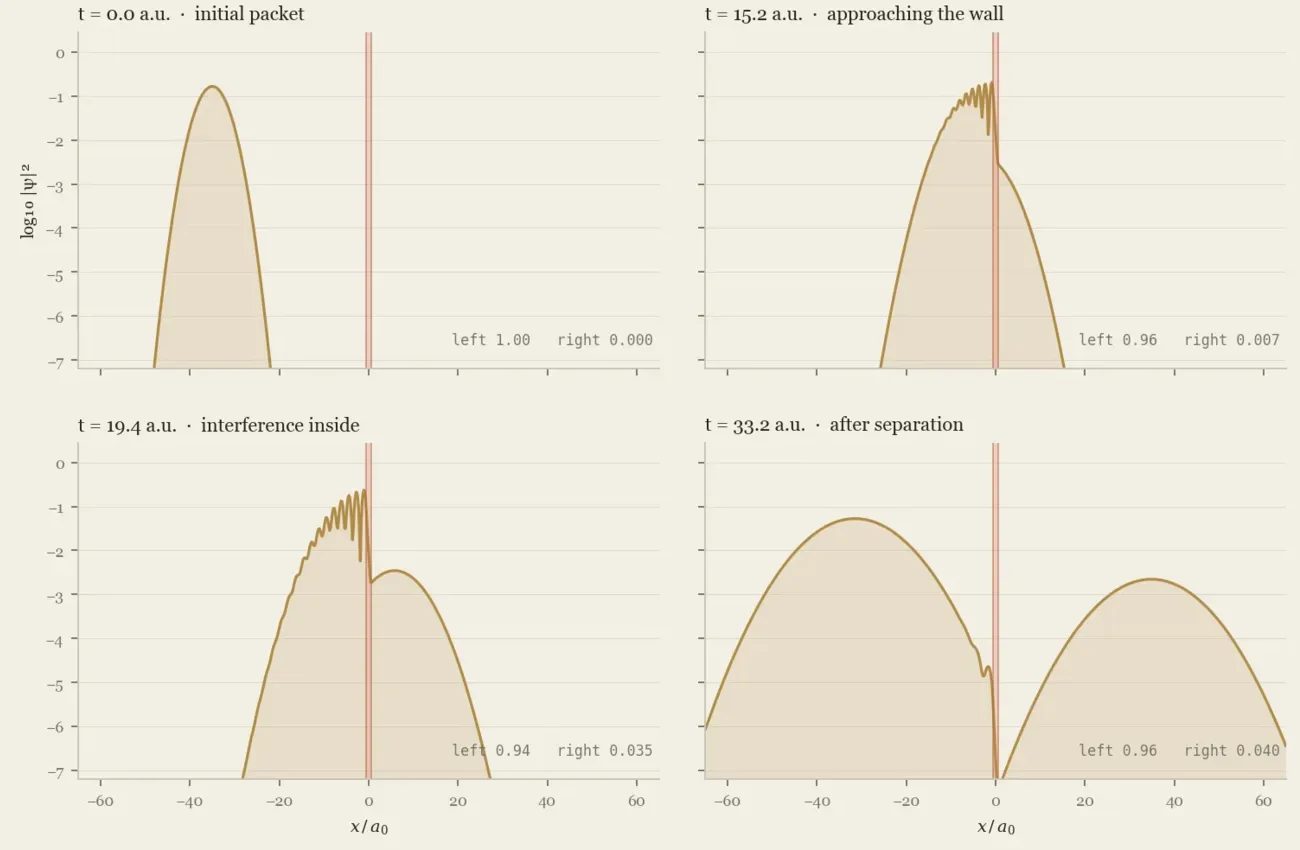
ψ(t+Δt) = e−iVΔt/2 𝓕⁻¹[ e−ik²Δt/2 𝓕[ e−iVΔt/2 ψ ] ]

Four snapshots of log probability density: a wave packet approaches a barrier, interferes with itself inside it, and splits into a reflected part (0.96) and a transmitted part (0.040).
Tunnelling

Fluid simulation

Small rules. Fluid behaviour.

How local particle interactions become fluid motion: smoothed particle hydrodynamics in C++, running here as WebAssembly.

C++ · OpenGL · SPH

SPH · neighbourhood study
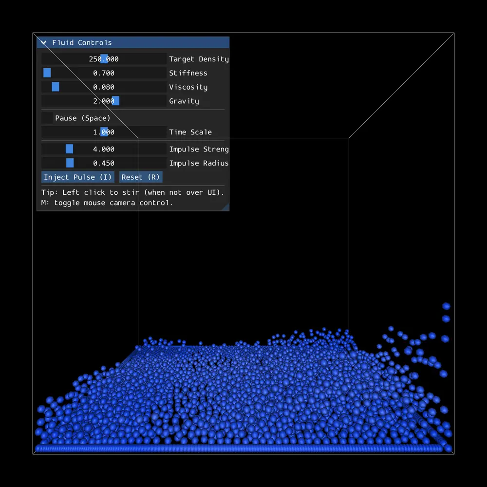
Fig. 003
A captured frame from the desktop build: the particle layer sloshing up the right wall.

N neighbours–

Drag to stir · click to splash · hover to see who counts

The interesting part happens between the particles.

Working prototype updated

Change the radius. See who counts.

02 Workbench

Code meets the physical world.

Circuits, mechanisms, and instruments.
Still being designed. Already teaching me things.

04 / Orion Design in progress
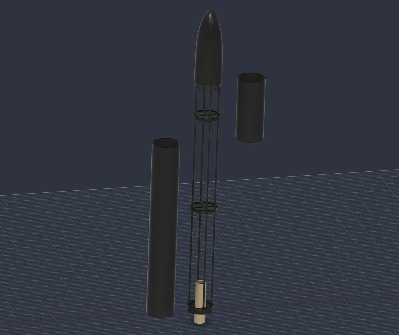
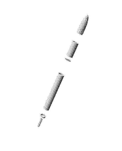
Orion line study: elevation, oblique and plan projections Projected from Orion_Master_V0.1.stl in the Orion repository, with hidden lines removed. Design only; nothing has been built.

learn to stay upright.

Orion

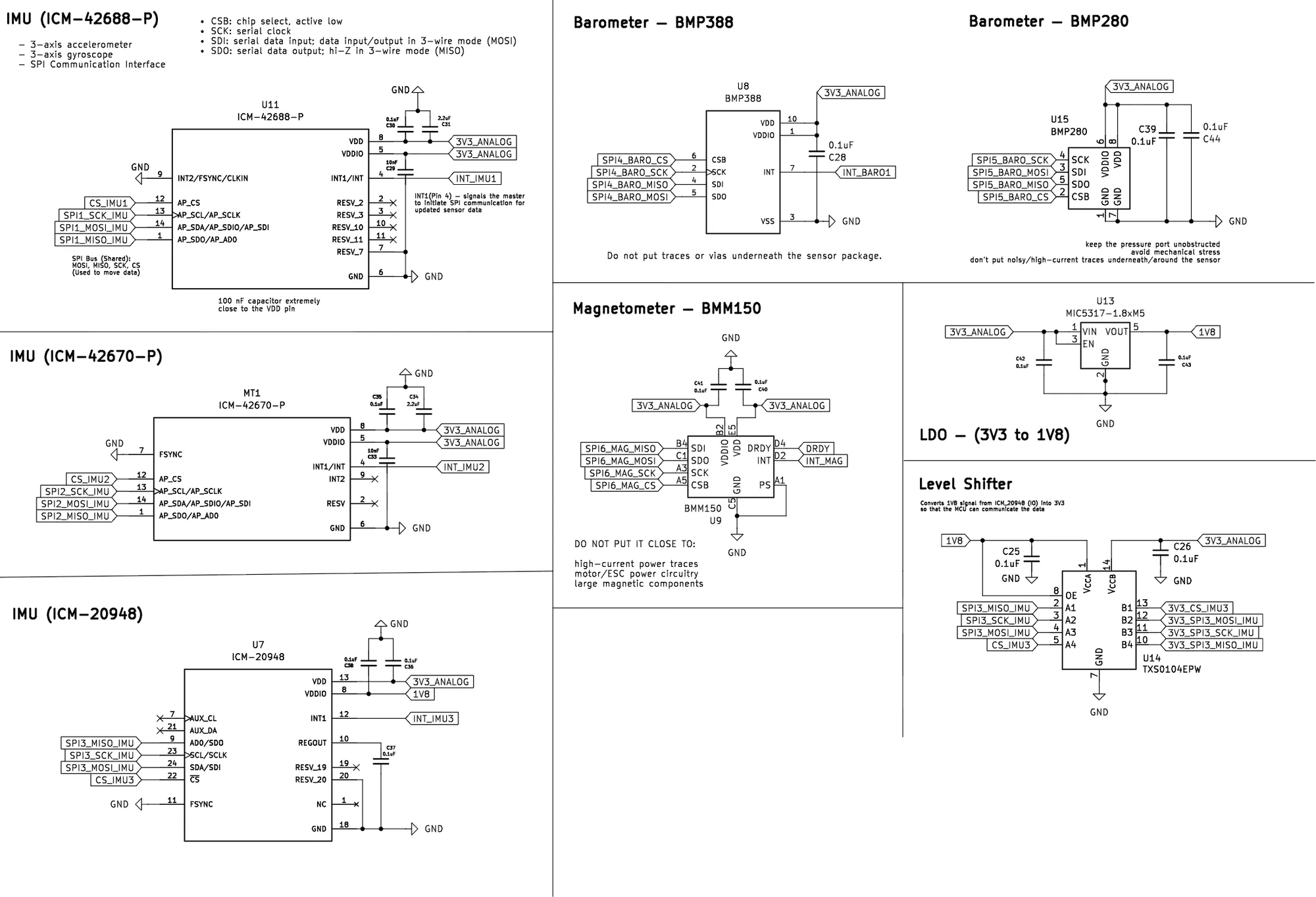
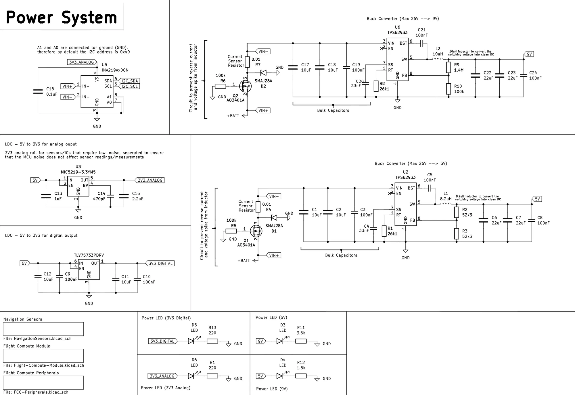
A flight computer. A gimbal. A lesson in control.

Custom avionics and a thrust-vector control mechanism for an actively stabilised model rocket.

KiCad / STM32 / Control theory

In progress updated

05 / Chladni plate Instrument design
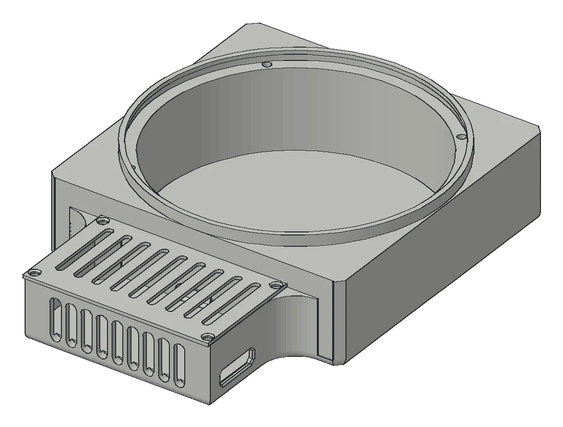
Chladni plate enclosure: oblique and plan projections Projected from enclosure_V2.stl and enclosure_cap.stl in the ChladniPlate repository, with hidden lines removed. Design only; nothing has been built.

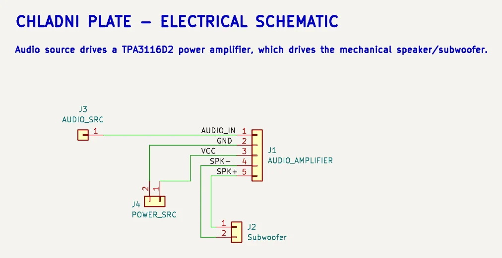
Seeing sound

Standing waves, made visible.

A custom enclosure and vibrating plate for finding patterns in resonance.

Acoustics / Electronics / Mechanical design

In progress updated

06 / ATLAS Planned · concept
ATLAS: conceptual hydrogen-line receive chainConceptual only. A one-metre dish focuses radio waves onto a feed, followed by a low-noise amplifier, a band-pass filter, a software-defined radio and a computer that looks for the 1420.4 megahertz hydrogen line. No components have been chosen.DISH · 1 mFEEDLNAFILTERSDR1420.4 MHz

Listening to hydrogen

A one-metre dish for the 21 cm line.

Radio / 1420 MHz / Astronomy

Planned updated

03 Scratchbook

The unfinished is interesting, too.

A few pages from the things I’m figuring out.
Some work. Some lead to better questions.

Experiment 01 / Dynamical systems

A little chaos

Lorenz attractor

How can a simple system become unpredictable?

Three coupled equations with σ = 10, ρ = 28 and β = 8/3, stepped with forward Euler at dt = 0.01. The notebook also covers phase space and the Van der Pol oscillator.

ẋ = σ(y − x) ẏ = x(ρ − z) − y ż = xy − βz

Python / Matplotlib

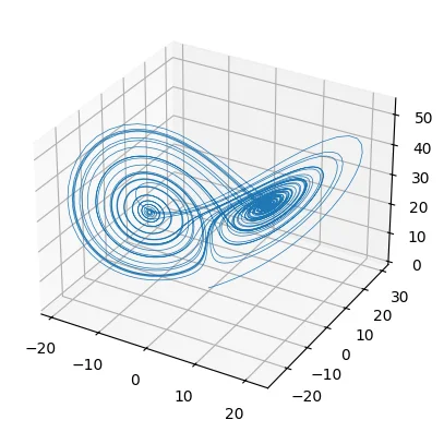
The Lorenz attractor plotted in three dimensions: two looping lobes traced by a single trajectory.
5,000 steps from (0.01, 0.01, 0.01), plotted with Matplotlib.
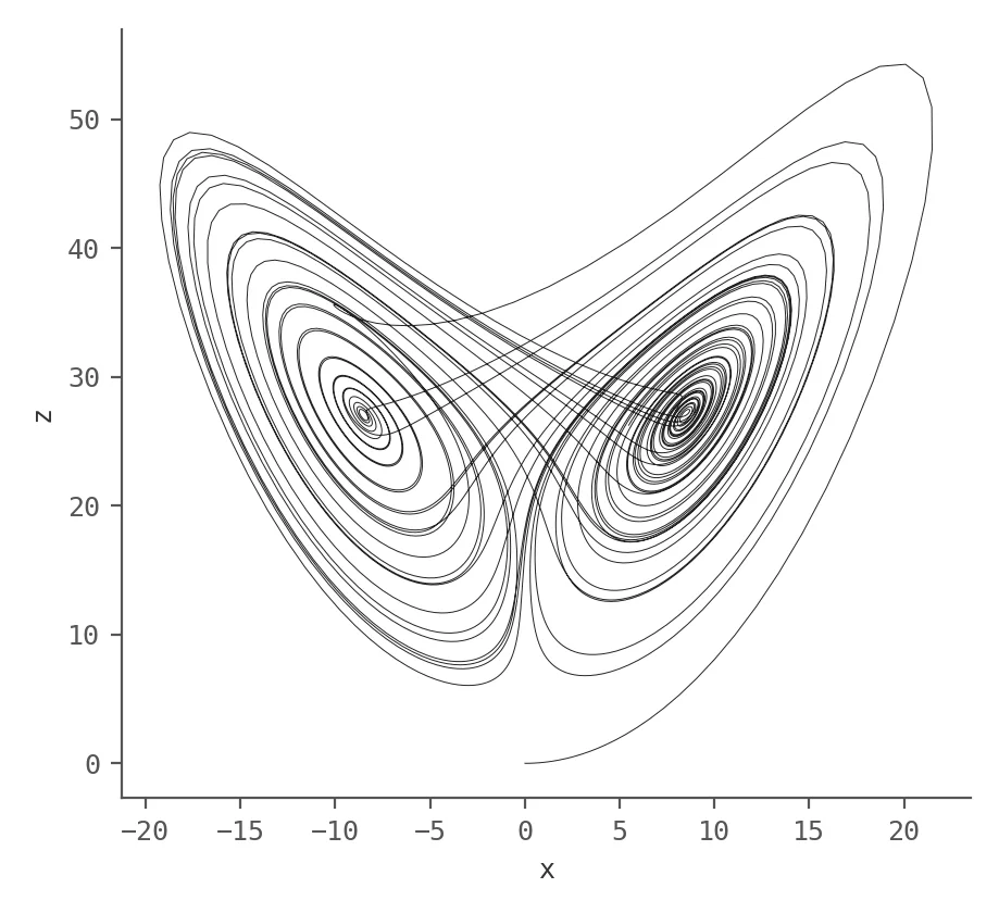
The Lorenz trajectory projected onto the x–z plane: two loops joined in a butterfly shape.
x against z
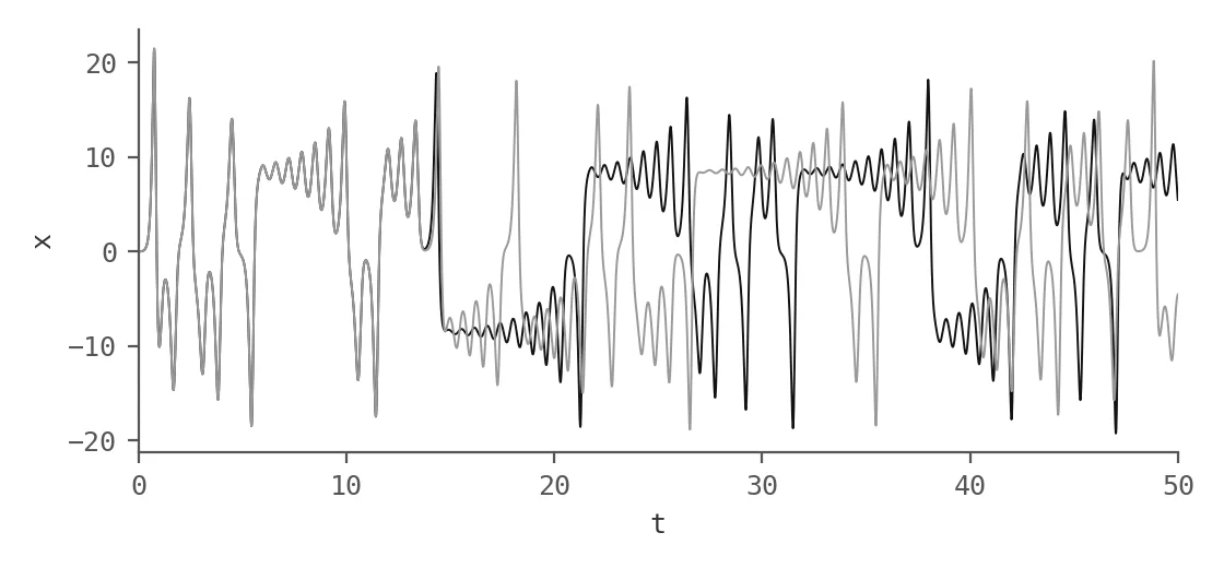
x over time for two runs that start 0.00001 apart; the two curves match until about t = 14, then separate.
Two starts 10⁻⁵ apart part ways near t = 14

chaotic is not the same as random

The trajectory never repeats and never settles, yet it stays on the same two-lobed shape. Bounded but unpredictable was the idea I wanted to see.

Open question How quickly do two starting points 10⁻⁵ apart stop agreeing?

Experiment 02 / Numerical integration

Everything pulls on everything

Particle simulation

What happens when particles only feel gravity and each other?

Particles fall toward a point with an inverse-square pull (softened below a distance of 5 so nothing divides by zero), bounce off each other with elastic collisions, and stay inside a sphere. Rendered with OpenGL; released for macOS, Linux and Windows.

C++ / OpenGL / GLM / CMake

Working prototype Open the project
void VerletIntegration(Particle3D& particle, float deltaTime){
  particle.position += particle.velocity * deltaTime
                     + 0.5f * particle.acceleration * deltaTime * deltaTime;
  glm::vec3 oldAcceleration = particle.acceleration;
  particle.acceleration = glm::vec3(0.0f);
  SetGravity(particle);
  particle.velocity += 0.5f * (oldAcceleration + particle.acceleration) * deltaTime;
}
ParticleSimulation/main.cpp
Order of operations in one velocity Verlet step A timeline from t to t plus delta t. Step 1 moves the position with the old velocity and acceleration, step 2 recomputes the acceleration at the new position, step 3 updates the velocity with the average of the old and new accelerations. t t + Δt 1 x += vΔt + ½aΔt² 2 a ← gravity(x) 3 v += ½(a_old + a_new)Δt
The three steps of one update, in the order the code runs them.

compare with the fluid sim's integrator

Velocity Verlet averages the old and new accelerations, so it needs the force evaluated twice per step. That ordering is the whole difference from the semi-implicit Euler loop in the fluid simulation.

Experiment 03 / Computational biology · hackathon

Reading the quiet genome

Myelovar

Which non-coding variants could plausibly matter in multiple myeloma, and why?

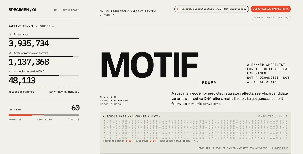
Seven stages, s0 to s6. Load the variants, drop common ones, keep those inside 18 ENCODE regulatory tracks from MM.1S myeloma cells, score transcription-factor motif disruption in a ±30 bp window, link each element to a target gene, weigh myeloma relevance with DepMap CRISPR data, then rank.

Python / FastAPI / React / 33 tests

Working prototype Open the project
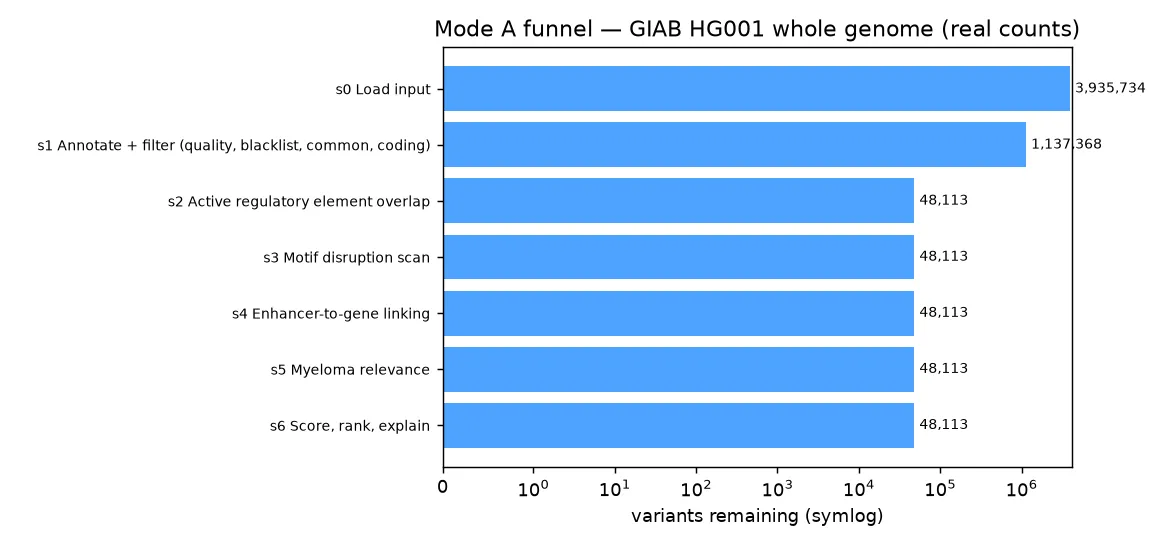
Funnel chart from the Myelovar web interface showing how many variants survive each pipeline stage.
Stage-by-stage variant counts from the pipeline's own funnel view.
The Myelovar review page: a variant funnel from 3,935,734 to 48,113 variants beside the Motif Ledger title, labelled illustrative sample data.
The review page, on sample data

research use only, not a diagnostic

Most of the work was making each filter explainable. Every surviving variant carries a plain-English evidence chain, so a reader can see which stage kept it and why.

Experiment 04 / Software · desktop assistant

An assistant I can read

Buffy

What would a personal assistant look like if I could read every line of it?

An Electron and TypeScript assistant that can run a local model through Ollama or Claude through the API. Every tool is tagged with a scope; reads run freely, while file deletions, shell commands and anything external wait for a click. A pause switch denies every call until it is turned off.

TypeScript / Electron / Vitest

In progress Open the project
const DEFAULT_RULES: Record<Scope, Decision> = {
  read: 'allow',
  local_write: 'allow',
  destructive: 'ask',
  external: 'ask',
  system: 'ask',
};

setRule(scope: Scope, decision: Decision): void {
  if (scope === 'external' && decision === 'allow') {
    throw new Error('External actions always require approval ...');
  }
  this.rules[scope] = decision;
}
src/core/permissions.ts
Sketch of Buffy's permission rules Five tool scopes on the left. read and local_write run immediately; destructive, external and system wait for approval. external is circled: the code refuses to set it to allow. runs asks first read local_write destructive external system external can never be set to allow
DEFAULT_RULES from the policy file, drawn as a flow.
Buffy’s Today view: a sidebar with Chat, Schedule, Tasks, Widgets, Approvals, Memory and Activity, a briefing card and a quick sticky note.
The Today view

Writing the policy as a small class with its own tests made the safety rule something I could check, rather than something I hoped the model would follow.

Experiment 05 / Machine learning

Watching a model learn

Machine learning notebooks

What is a model actually doing when it learns?

Linear regression by gradient descent and by the normal equation, plus logistic regression, written with NumPy and pandas instead of a machine learning library.
θ = (XᵀX)⁻¹ Xᵀy

Python / NumPy / pandas / Jupyter

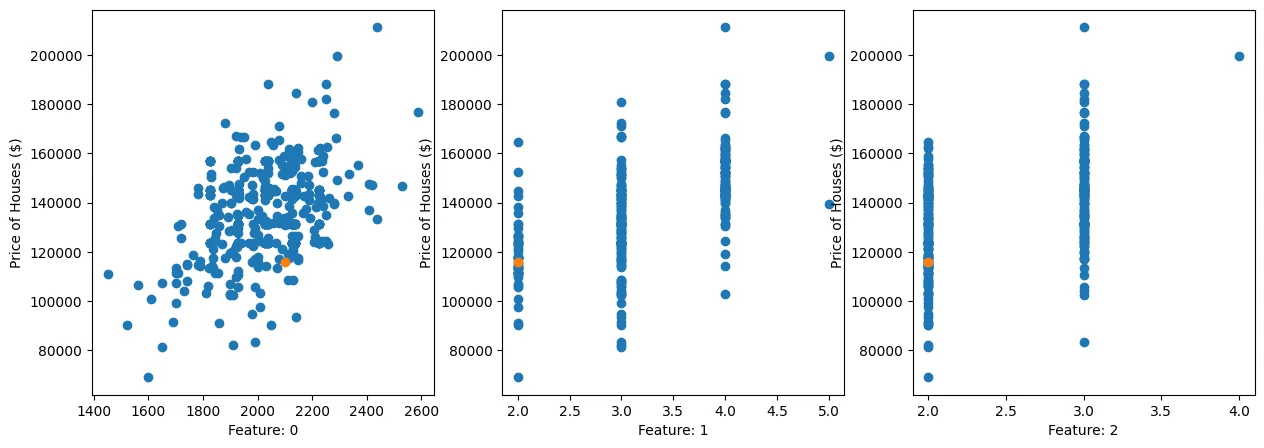
Three scatter plots of house price against square footage, bedrooms and bathrooms, with one predicted house highlighted in orange.
Normal-equation fit on house_prices.csv; the orange point is the prediction for 2,100 sq ft, 2 bedrooms, 2 bathrooms.
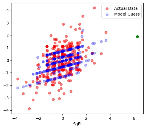
Scatter plot of scaled house price against square footage: actual prices in one shade, the model’s guesses in another along a rising band.
Guesses against prices, by size

The normal equation gives the answer in one line of linear algebra, which made it obvious what gradient descent is iterating toward.

04 Writing

Explaining it to understand it.

Schrödinger's Equation for Dummies

  1. Part I · 9 min read

    Historical Overview (Schrödinger's Equation for Dummies, Part I: Historical Overview, on Medium)

    · Medium · companion to QuantumSim

  2. Part II · 8 min read

    Decoding the Equation (Schrödinger's Equation for Dummies, Part II: Decoding the Equation, on Medium)

    · Medium · companion to QuantumSim

About

Student in Brampton, Ontario. Physics, maths, code, electronics. Founder of CodeCraft Academy; programmer for FRC Team 1325.